
Take the web UI for a spin
The web UI is the browser face of the same bitemporal engine the
TUI drives. It trades the terminal for things a
terminal can’t do well: a force-directed topology graph, shareable
deep-links (/history?mac=…), and a click-through from a VM to the
physical switchport it lives on. Sixteen screens, one nav rail, and a
time control that scrubs both axes of the bitemporal model at once.
It’s a two-tier split. A static Astro build (sixteen pages, each mounting
one React island) talks to a read-only FastAPI over /api/*. In
production a single container serves the built frontend and the API,
so the same image works with or without SSO — auth is entirely
server-side.
Bring it up
Section titled “Bring it up”The UI ships as a compose overlay that serves the built frontend and the read API as one service behind your reverse proxy:
docker compose -f docker-compose.yml -f docker-compose.web.yml up -d --build webIt comes up at the hostname in the service’s caddy label (override
with L2TRACE_WEB_HOST); the API stays read-only, and Postgres/NATS
stay off the shared network. Everything you see below was captured
against the realistic seed — bring the same
data up with make seed-realistic followed by make seed-web-extras
(the second one adds the vSphere correlations, an unknown neighbor, and
a quarantine burst that light up the last three screens).
For hot-reload hacking, run the API with uv run l2trace web and the
Astro dev server with pnpm --dir web-ui dev — Vite proxies /api to
the backend, so edits to either side reload on save.
The time circuits — bitemporality you can scrub
Section titled “The time circuits — bitemporality you can scrub”Every data screen carries the same control at the top. Collapsed, it’s a one-line strip; click it and it unfolds into a dashboard modeled on the DeLorean’s time circuits, because it’s doing exactly what that prop implied — moving through two independent time axes at once.
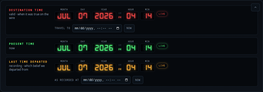
- DESTINATION TIME (red) is valid time — when a fact was true on the wire. “Travel to” 3pm last Tuesday and every screen answers as of the network’s state then.
- PRESENT TIME (green) is a read-only live clock, ticking every second, so you always see where “now” sits relative to the two dials.
- LAST TIME DEPARTED (amber) is recording time — which belief snapshot you departed from. Set it to ask “what did the system believe last Tuesday,” before a late-arriving event revised the record.
A dial reading LIVE tracks now; set it and it flips to SET. Leaving
both live is the default — you’re looking at current truth, current
belief. This is the one control that makes the difference between “where
is MAC X” and “where did we think MAC X was, as of a belief we held an
hour ago” a matter of two clicks. The concept is spelled out in
Querying past beliefs and
Bitemporality.
Trace — hop-by-hop path
Section titled “Trace — hop-by-hop path”The landing screen. Enter a source MAC, a destination MAC, and a VLAN.
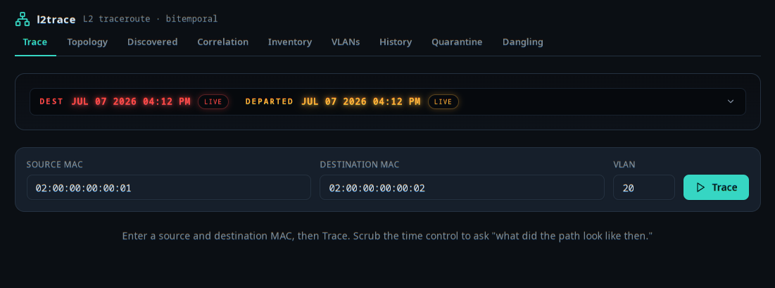
The MAC and IP fields (here, and on Diff and History) autocomplete on
identifiers l2trace has actually observed: start typing and a dropdown offers
matching MACs (hinted with their OUI vendor) and IPs (hinted with their bound
MAC). Matching is format-insensitive, so 001b, 00:1b, and 00-1b all find
the same prefix. Suggestions are a convenience, not a constraint: a MAC the
fabric has never seen still submits, which matters when you are chasing
something new.
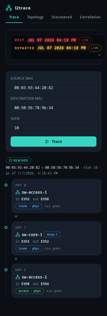
Run it and the path renders as a vertical timeline, one card per hop: the device, the ingress port (where the frame entered) and egress port (where it leaves toward the next hop), the port role (access vs trunk), and the source that vouched for that CAM entry.
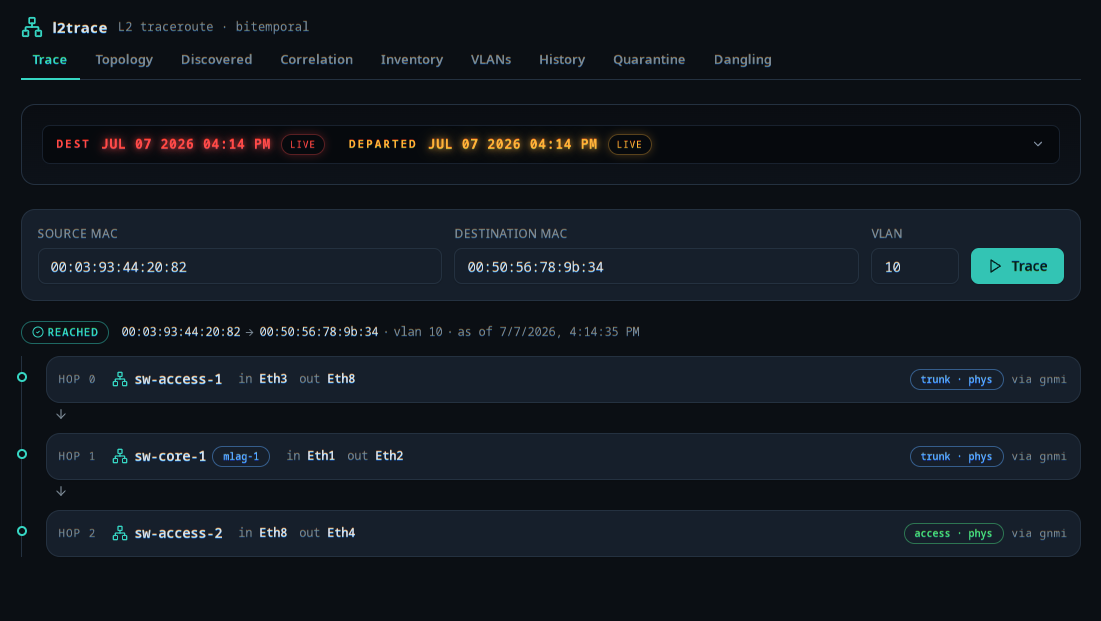
The badge up top is the termination reason — why the trace stopped.
reached (green) is the happy path. floods, dead-end, loop, and
too_many_hops each tell you where the reconstruction gave up rather
than silently returning nothing. When the path crosses an MLAG pair,
the core hop wears an mlag-N badge — the peer pair is collapsed to one
logical node so a dual-homed link doesn’t read as a flap. See
the traceroute algorithm and
MLAG collapse.
Scrub the time circuits while a result is on screen and the trace re-runs at the new moment — no retyping.
Diff — did the path change between two times?
Section titled “Diff — did the path change between two times?”Trace answers “where does this frame go now.” Diff runs the same
reconstruction at two belief times and aligns them hop-by-hop, so you can
ask “did anything move between 3pm and now, and where.” Enter the src
and dst MAC, the VLAN, and two times — t1 (before) and t2 (after),
each accepting ISO-8601 or a relative now-30h / now-2d.
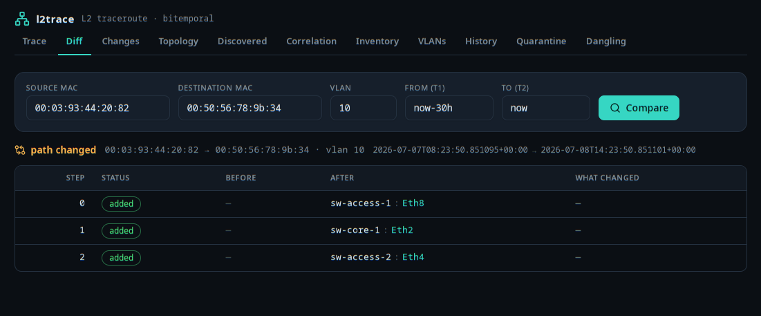
The headline says path unchanged or path changed at a glance; the
table then breaks it down per step. Each hop is coloured by status —
unchanged, changed (the port or device differs between t1 and t2),
added (this hop only exists at t2), or removed (it was there at t1
and is gone). The before and after columns carry the hop as it stood
at each time, so a shifted egress port or a re-homed uplink is right
there in the row. The capture above is a path that came into existence
between the two times — every hop added, because at t1 the source
hadn’t appeared yet (no_ingress) and by t2 the full three-hop path
reaches. A moved endpoint instead produces a changed row with both
sides populated. This is the l2trace trace-diff CLI
query with a form on top.
Changes — what churned on the fabric
Section titled “Changes — what churned on the fabric”Where Diff targets one path, Changes is the fleet-wide review: pick a window (24h / 7d / 30d) and see everything the bitemporal log says happened in it, in four sections.
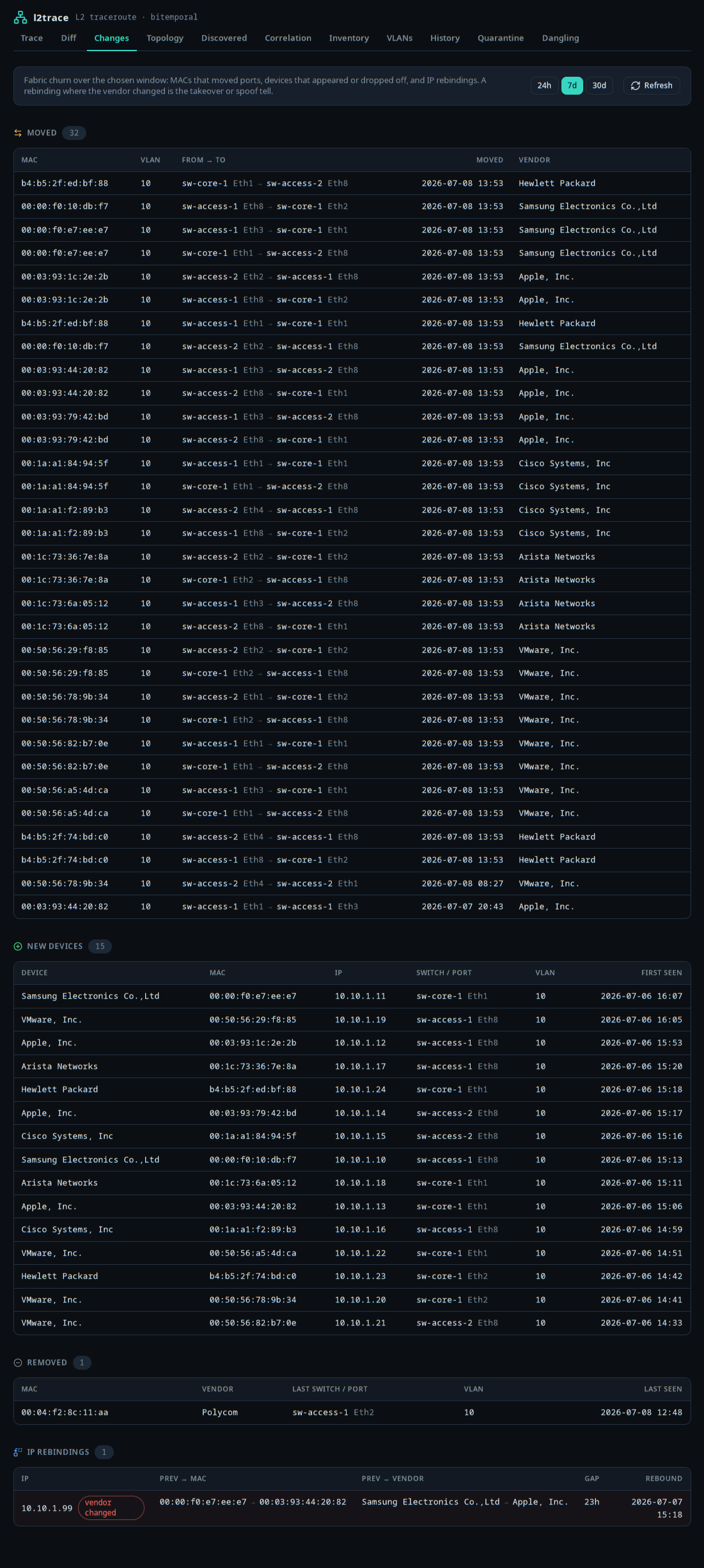
- Moved — a MAC seen on a different (switch, port) than immediately before. A frame learned across the fabric’s trunks in one sweep registers a move on each hop it propagates through, so real churn on a busy fabric fills this table quickly.
- New devices — MACs whose earliest-ever sighting lands in the window: something new plugged in.
- Removed — MACs whose last sighting closed in the window with no open successor: something unplugged or decommissioned.
- IP rebindings — an IP that swapped the MAC bound to it. Most are
benign DHCP churn, but the one flagged vendor changed (red, pulled
to the top) is the tell that matters: a DHCP renewal keeps the same MAC
and vendor, so a different-vendor MAC claiming an address is what an
ARP-spoof or takeover looks like. In the capture,
10.10.1.99jumped from a Samsung MAC to an Apple one.
Every count is drawn from current-belief rows, so a correction that arrived late reads as the corrected reality, not the original mistake.
Topology — the fabric as a graph
Section titled “Topology — the fabric as a graph”A force-directed map of devices (nodes) and resolved LLDP/CDP adjacencies (edges). Node shape and color encode kind; a double border marks an MLAG pair.
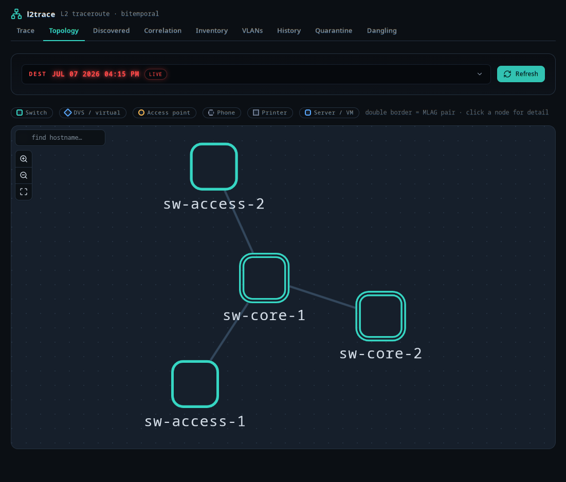
Endpoints (phones, APs, printers, servers) are hidden by default so the fabric reads clearly — the per-category toggles in the legend reveal them on demand, each refetching just its slice. Search a hostname, or click any node for a detail card: type, role, vendor, link count, instrumentation visibility, and MLAG group.
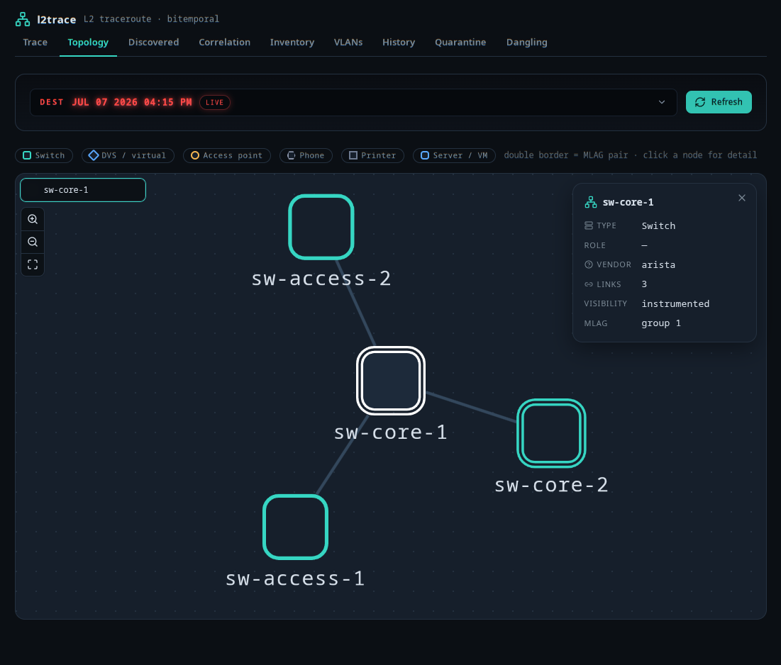
Only adjacencies whose peer port resolved become edges. Neighbors the graph can’t place yet don’t vanish silently — they surface on the Dangling screen.
Discovered — what’s plugged into which port
Section titled “Discovered — what’s plugged into which port”Every endpoint forwarding on an access port right now, joined across CAM, ARP, the IEEE OUI registry, and vSphere placement. Uplinks and infrastructure are excluded, so this is the direct answer to “what is plugged into which port?”
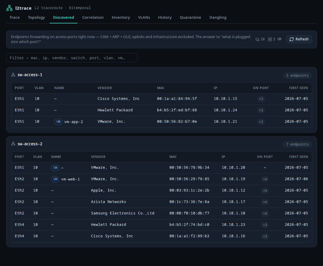
Grouped by switch, sorted by natural port order (Gi1/0/2 before
Gi1/0/10). VMs get a badge; a ×N in the on port column flags a
shared/trunk port carrying more than one MAC. This is the same feed the
Nautobot SSoT app consumes to propose device
shells — here it just answers the operator question directly.
Correlation — VM ↔ physical switchport
Section titled “Correlation — VM ↔ physical switchport”The join vCenter can’t give you alone: a vSphere VM MAC that also shows up in an SNMP CAM table. Each row is one cross-confirmed MAC — the VM side (name, ESXi host, dvPortgroup VLAN) bridged to the physical side (switch, port, CAM-learned VLAN).
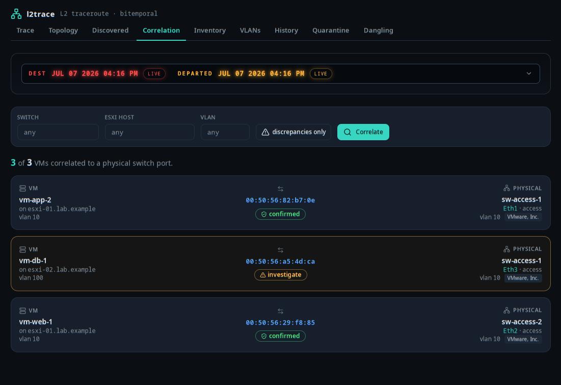
The confidence badge is the point. confirmed means both sides agree.
investigate (amber) means the VLANs differ — legitimate on a trunk,
where vSphere reports the dvPortgroup VLAN and the switch reports what
it learned, but worth a look. stale means one side has aged out. The
“discrepancies only” toggle narrows to just the rows worth chasing;
click any row to jump to that MAC’s history.
Inventory — count the fleet
Section titled “Inventory — count the fleet”A pivot over every currently-observed MAC. Group by vendor, VLAN, or port role; each row is a proportion bar with the MAC count and the switch/VLAN spread.
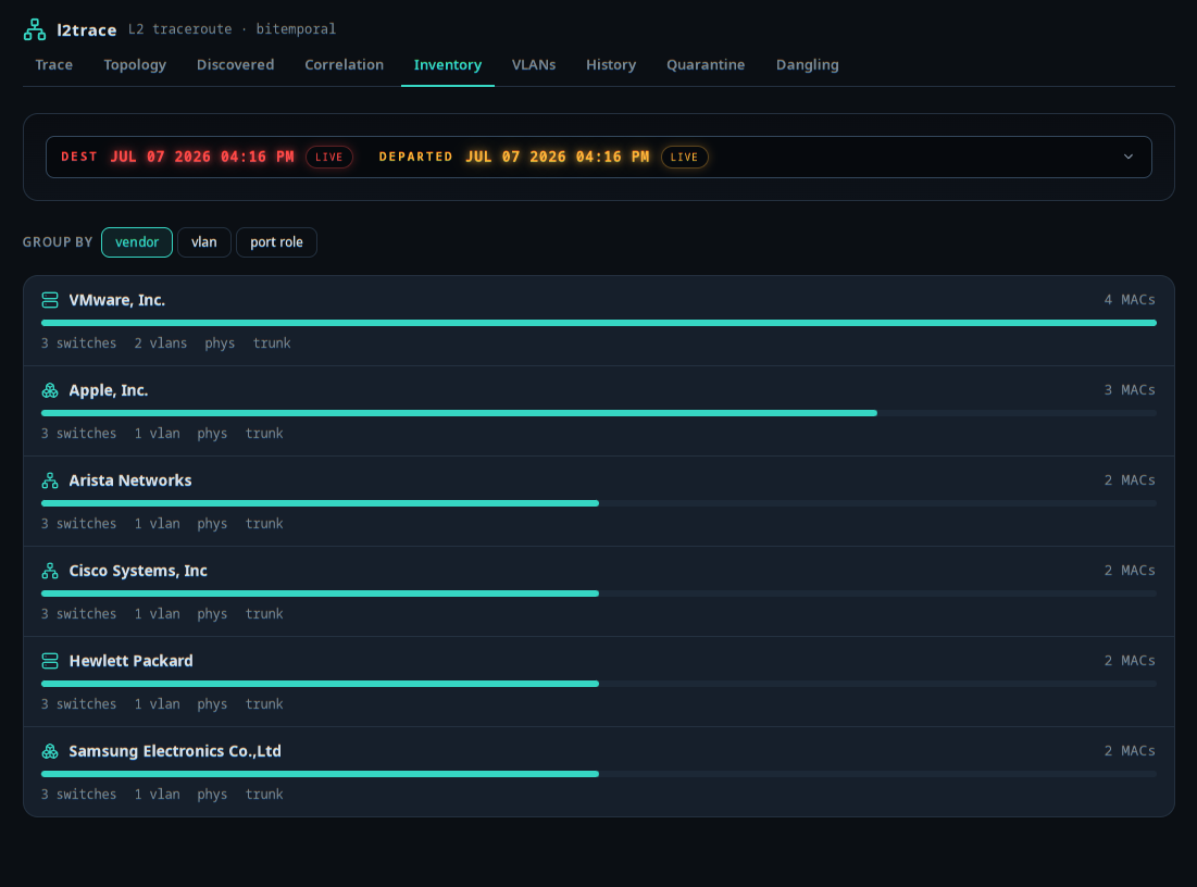
Vendor families get a recognizable icon (printer, camera, phone, server…), but that’s presentation only — the authoritative axis is always the IEEE organization string, never the glyph.
VLANs — the segmentation map
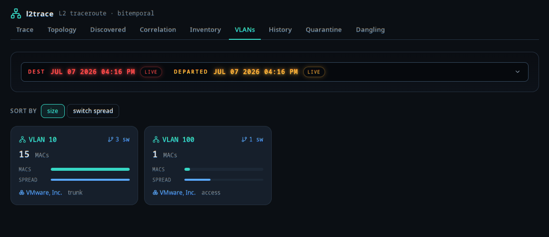
Section titled “VLANs — the segmentation map”The VLAN pivot lifted into its own screen: one card per VLAN, sortable by size (MAC count) or switch spread (how many switches carry it). A VLAN living on many switches is a broadcast domain worth understanding; one stuck on a single switch might be a leftover.
History — one endpoint’s whole life
Section titled “History — one endpoint’s whole life”Search a MAC — or an IP, which resolves to its MAC via ARP/ND and wireless bindings first — to see every port and VLAN it has lived on, newest first.
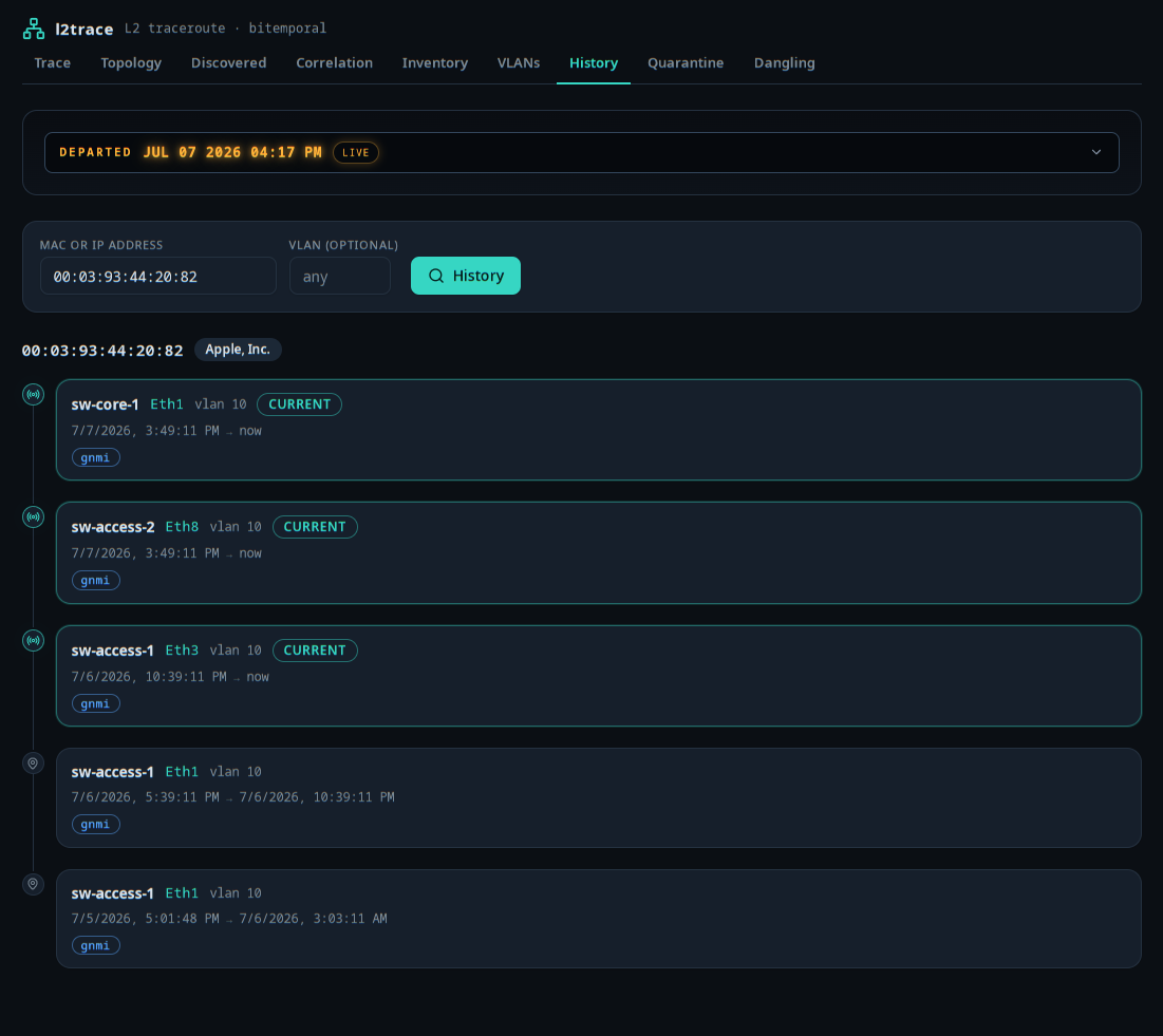
Open tenancies pulse and wear a current badge; closed ones show their
[first seen → last seen] window. Note the time control here carries
only the amber LAST TIME DEPARTED axis — history is inherently a
walk through valid time, so the axis you’d scrub is belief: “what did
we believe this MAC’s history was, as of last week?” The MLAG-heavy seed
shows the same MAC as current on a core trunk and an access edge at once
— that’s a frame traversing the fabric, not a contradiction.
Quarantine — events the reconciler refused
Section titled “Quarantine — events the reconciler refused”The reconciler won’t ingest an event whose timestamps fail a trust check; instead of dropping it, it parks it on a NATS stream for review. This screen peeks that stream without consuming it — nothing here has touched the database. The landing view is one card per device.
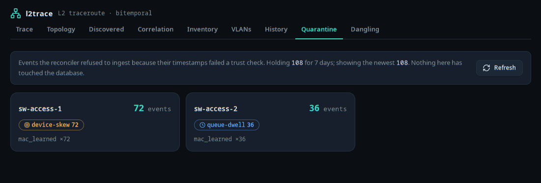
Two reasons, color-coded because they point at different culprits: device-skew (amber) means the device’s clock disagrees with the collector’s beyond budget — check NTP on the device. queue-dwell (blue) means the event sat too long between collector publish and reconciler ingest — check the pipeline, not the device. Click a device to drill in; the burst collapses to one row per distinct payload with a repeat count and a plain-English “why it was rejected.”
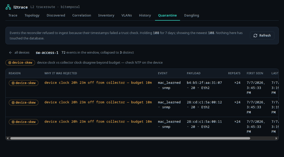
See how to spot disagreements for the device-clock-vs-queue-dwell distinction in depth.
Dangling — edges the graph can’t draw
Section titled “Dangling — edges the graph can’t draw”The other side of Topology: LLDP/CDP neighbors visible on the wire that never became a drawable link, split by why.
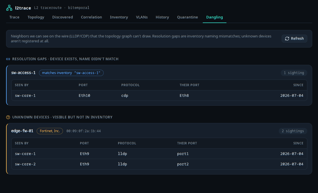
Resolution gaps are neighbors whose advertised sysname matches an
inventory hostname that just didn’t link — a naming mismatch to
reconcile, not a mystery. Unknown devices aren’t in inventory at all;
the one visible here is identified only by its chassis MAC’s OUI
(Fortinet, Inc.) and the two core ports that see it — enough of a lead
to go register it. Grouping is by neighbor identity, so one device seen
from seventeen ports reads as one card with a sightings table, not
seventeen cards. Why unresolved rows are excluded from the graph is
covered in peer resolution.
Rogues — wireless intruders, split by what you can do
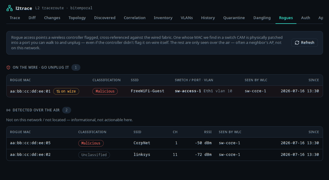
Section titled “Rogues — wireless intruders, split by what you can do”A wireless controller flags rogue APs it hears over the air; this screen cross-references those MACs against the wired fabric and sorts them by whether you can act. On the wire · go unplug it is the actionable set — a rogue MAC found in a switch CAM is physically patched into a port, so the switch, port, and VLAN are spelled out for you to walk over and pull it. That the controller didn’t flag it on-wire itself doesn’t matter; a CAM hit is the stronger signal. Detected over the air is everything else — often a neighbor’s AP, shown with channel and RSSI but not on this network, so informational rather than something to chase. The classification badge (malicious, friendly, or unclassified) rides along from the controller, and the malicious ones sort to the top.
Rogue Switches — unmanaged gear on the edge
Section titled “Rogue Switches — unmanaged gear on the edge”Where Rogues is wireless, Rogue Switches is the wired equivalent: edge ports that look like an unauthorized switch or hub was plugged in, sorted worst-first into two categories. Unmonitored switches announce themselves over LLDP/CDP but have no collector behind them — l2trace can see them yet doesn’t poll them, and a neighbor that matches nothing in inventory at all is the strongest flag. Silent hubs announce nothing; their only tell is a pile of MACs learned on one access port, so the row leans on the MAC count and the spread of distinct vendor OUIs to judge whether it’s really a downstream switch (many vendors) or just a multi-NIC host or hypervisor (one OUI, scored down). A min-MACs control (2 / 3 / 5) sets how many MACs a silent port needs before it’s flagged; unmonitored switches are flagged regardless of count. High-confidence rows carry a red border, and each row’s reasons spell out why it was called switch-like.
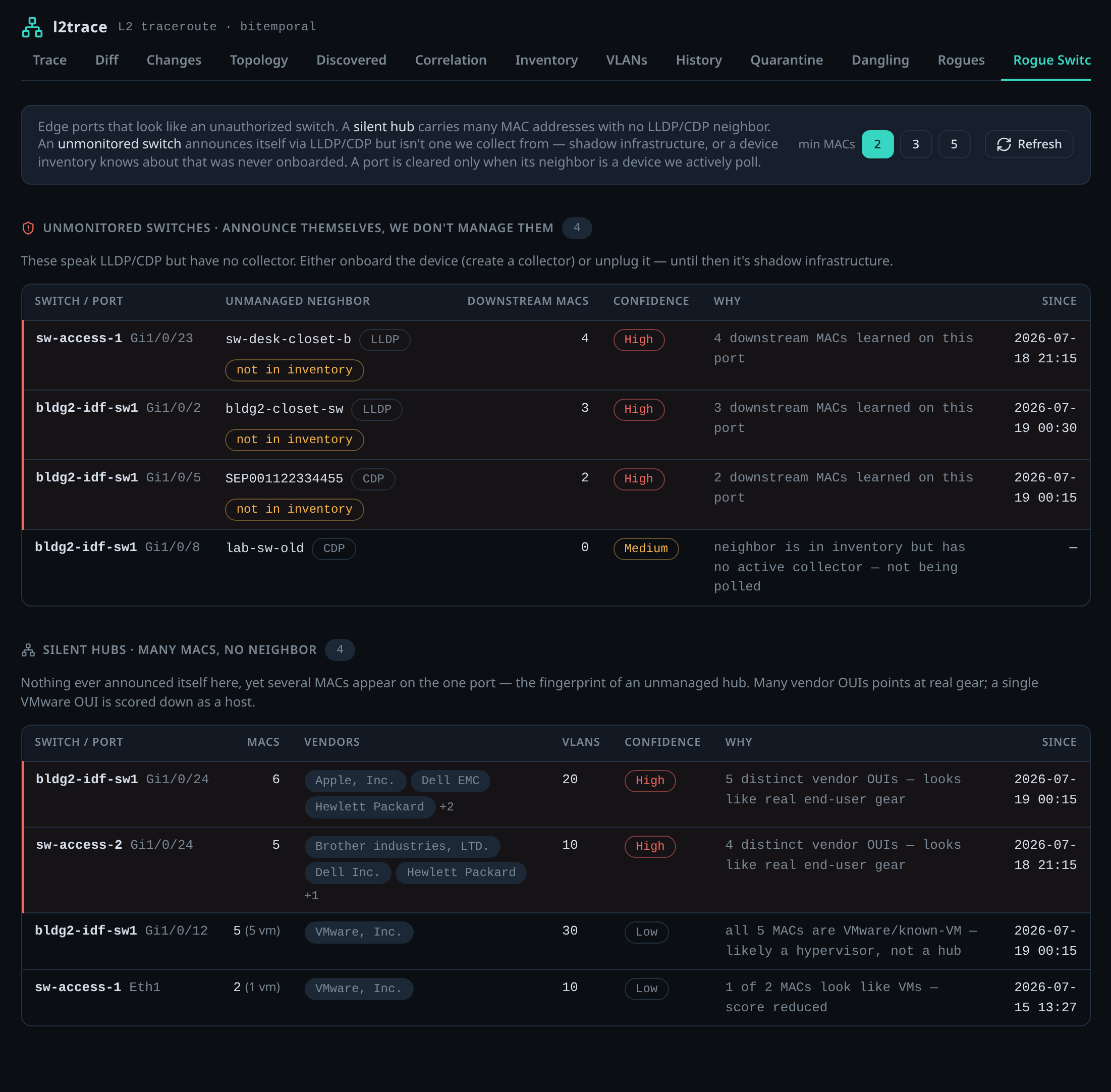
This screen reads current belief only — the time circuits don’t drive it — because “what looks unmanaged right now” is a live question, not a historical one. The task version is find an unmanaged switch; the reasoning is in how the detector decides.
Auth — 802.1X decisions, pinned to the port
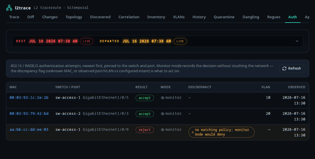
Section titled “Auth — 802.1X decisions, pinned to the port”Recent 802.1X / RADIUS Access-Request decisions, newest first, each anchored to the NAS switch and port it arrived on. The default posture is monitor — the server records the accept or reject it would return and changes nothing on the wire — so the value isn’t the verdict but the discrepancy flag beside it: an unknown MAC, or an observed port/VLAN that disagrees with configured intent. Flagged rows pull an amber left border, and each MAC deep-links to its History. This screen carries the full time circuits, so you can read the auth log as of any belief you held.
Approvals — decide what gets onto the network
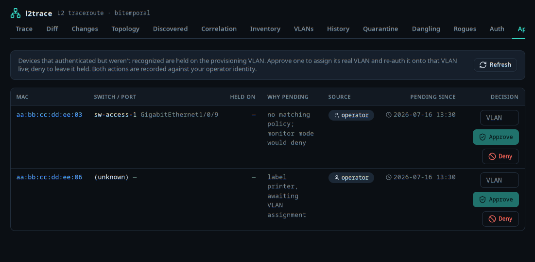
Section titled “Approvals — decide what gets onto the network”The one screen that writes. Devices that authenticated but weren’t
recognized sit held on a provisioning VLAN, each row waiting on you.
Type the real VLAN and Approve to assign it and fire a live CoA
re-auth that moves the device onto it — or Deny to leave it held.
Both actions record against your operator identity, so this is the one
place the read-only rule bends; both need a signed-in operator, and a
401 means “sign in first,” not a fault. When Nautobot’s synced intent
disagrees with an explicit operator decision, a banner lists the
conflicts — neither side is reconciled automatically, so you re-decide
to settle it.
Search — one box over everything
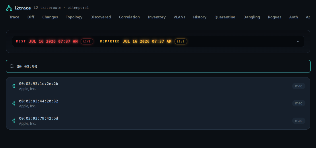
Section titled “Search — one box over everything”A single field across every identifier l2trace has seen: device hostnames, management IPs and chassis MACs, port names, observed MACs, ARP-bound IPs, LLDP/CDP neighbor sysnames, and rogue SSIDs. Results come in as you type (two-character minimum), each tagged by kind and deep-linked to the screen that can show it — a MAC to its History, a device to Topology. It honors the time circuits too, so a search runs as of whichever moment the dials hold: you can look for a hostname the fabric carried last Tuesday, not just now.
It works on a phone
Section titled “It works on a phone”The whole thing is mobile-first. The nav rail scrolls horizontally instead of collapsing into a hamburger (every destination stays one thumb-flick away), the trace form stacks, and the hop timeline reflows into a single column.
A note on auth
Section titled “A note on auth”The build is identical with or without SSO. When OIDC_ENABLED is set,
the server installs an OpenID Connect gate (tested against Authentik) and
a signed-in user chip appears top-right; when it isn’t, the app serves an
anonymous shim and the chip renders nothing. Front it with your reverse
proxy for TLS either way.
Regenerating these screenshots
Section titled “Regenerating these screenshots”Every image on this page is captured by scripts/web_screenshots.py
(Playwright) against a seeded stack. With the API and Astro dev server
running:
make web-screenshotsIt drives each screen, waits for the data to settle on the view’s
accessibility landmark (not a blind timer), and writes PNGs into
docs-site/public/screenshots/web/. Re-run it after a UI change to keep
the docs honest.
What’s next?
Section titled “What’s next?”- The other interface: Take the TUI for a spin
- The concept under the time circuits: Querying past beliefs
- Investigate a real MAC: How to investigate a MAC’s history